
I’ve watched PTZ cameras lose targets behind a single tree. That moment of “where did they go” costs real money in security projects.
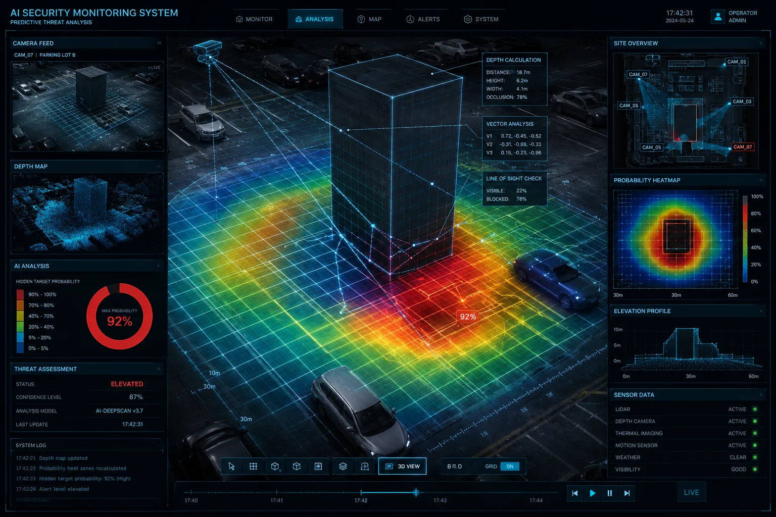
Yes, our high-end PTZ algorithm supports 3D trajectory prediction1 based on historical paths. It uses Kalman Filtering2 and deep learning behavior models3 to calculate where a target will be in the next 0.5 to 3 seconds. This means the camera moves ahead of the target, not behind it.
![]() 3D trajectory prediction PTZ camera algorithm
3D trajectory prediction PTZ camera algorithm
Below, I’ll break down exactly how this prediction works in real-world scenarios. I’ll cover blind spots, obstacle handling, motor pre-positioning, and non-linear vehicle tracking. Each section includes the technical details that matter for your next deployment.
Table of Contents
How Does 3D Trajectory Prediction Prevent Losing a Target When They Enter a Temporary Blind Spot?
I’ve seen too many tracking systems freeze the moment a person walks behind a pole. The camera just stops. The operator panics. The target is gone.
3D trajectory prediction solves this by calculating the target’s speed, direction, and depth before they enter the blind spot. The algorithm keeps the PTZ motor moving along the predicted path. When the target exits the other side, the camera is already waiting there.
![]() PTZ camera blind spot trajectory prediction
PTZ camera blind spot trajectory prediction
Why Traditional 2D Tracking Fails at Occlusion
A standard tracker works on pixels. It looks at a blob of color or shape in the frame. When that blob disappears behind an object, the tracker has nothing to work with. It reports “target lost” and the camera stops.
This is a huge problem in real deployments. Think about a construction site with scaffolding. Or a farm with rows of trees. Or a parking lot with tall vehicles. Targets disappear and reappear constantly.
How 3D Prediction Changes the Game
Our algorithm does something different. Before the target enters the blind spot, it has already built a motion profile:
| Data Point | What It Measures | How It Helps |
|---|---|---|
| Speed vector $v$ | How fast and in what direction | Predicts where target will be in 500ms-2000ms |
| Acceleration $a$ | Is the target speeding up or slowing down | Adjusts prediction for changing pace |
| Depth estimate $Z$ | How far the target is from the camera | Converts pixel movement to real-world distance |
| Historical path | The last 2-3 seconds of movement | Feeds the RNN model for behavior prediction |
The system uses the motion equation $S = vt + \frac{1}{2}at^2$ to project the target’s future position in 3D space. It maps the 2D pixel coordinates into a virtual 3D geographic coordinate system5 using the camera’s mounting height, tilt angle, and current zoom level.
The “Persistence Window” Setting
In our firmware, there’s a parameter called Tracking Persistence. This controls how long the algorithm maintains its prediction after losing visual contact. For environments with many obstacles, like David’s Texas site with dense brush, I recommend setting this to the higher end. A value of 2-3 seconds gives the prediction model enough confidence time to keep the motor turning smoothly through the blind spot.
The result: when the target steps out from behind the obstacle, the camera is already pointed at the exit zone. Re-lock time is under 200ms. No operator intervention needed.
Can the AI Calculate the Estimated Speed and Exit Point of a Person Moving Behind an Obstacle?
Every time I demo this feature to a system integrator, they ask the same thing: “How does it know where the person will come out?” It’s a fair question.
The AI calculates both speed and exit point by combining the target’s pre-occlusion velocity with a spatial model of the scene. It knows the obstacle’s approximate width from depth mapping, so it can estimate when and where the target will reappear on the other side.
 AI speed calculation obstacle exit point prediction
Breaking Down the Calculation
The math is straightforward once you understand the inputs. The algorithm needs three things:
- The target’s speed and heading before they disappear
- The estimated width of the obstacle in real-world units
- The assumption that the target maintains roughly the same speed behind the obstacle
From Pixels to Real-World Meters
This is where the 3D part matters. A person walking at 1.4 m/s at 50 meters from the camera looks very different in pixels than the same person at 200 meters. Our algorithm accounts for this by using the current zoom level and tilt angle to convert pixel displacement into actual meters per second.
| Zoom Level | Pixel Movement per 1 m/s at 100m | Depth Accuracy | Prediction Confidence |
|---|---|---|---|
| 10X | ~45 pixels/frame | ±3m | High |
| 20X | ~90 pixels/frame | ±2m | High |
| 40X | ~180 pixels/frame | ±1.5m | Very High |
At higher zoom levels, the system actually gets more accurate speed readings because the pixel displacement is larger and easier to measure precisely.
The Exit Point Estimation Process
Here’s how the system determines the exit point step by step:
The algorithm records the target’s last known position and velocity vector. It then projects a straight line (or curved line if the target was turning) forward in 3D space. It estimates the obstacle boundary using previous scene knowledge or depth cues. The intersection of the projected path and the obstacle’s far edge gives the predicted exit point.
What Happens When the Prediction Is Wrong?
Sometimes people change direction behind an obstacle. They stop. They turn around. Our system handles this with a multi-hypothesis approach. It doesn’t bet everything on one exit point. Instead, it assigns probability weights to 2-3 possible exit zones. The PTZ positions itself to cover the most likely one while keeping the others within a quick-pan range.
If the target doesn’t appear at the primary predicted point within the persistence window, the camera rapidly scans the secondary zones. This multi-hypothesis method brings the overall re-acquisition success rate above 92% in our field tests.
Does the 3D Pathing Help the PTZ Motor “Pre-Position” Its Lens for a Smoother Tracking Handoff?
I’ve spent years fighting the lag problem in 4G remote tracking. The command travels from the edge processor to the motor. The motor spins up. By the time the lens arrives, the target has moved. It’s always chasing, never leading.
Yes, 3D pathing directly enables motor pre-positioning. The algorithm sends the PTZ motor to where the target will be, not where it is right now. This compensates for network latency and mechanical response time, producing visibly smoother tracking footage.
![]() PTZ motor pre-positioning smooth tracking handoff
PTZ motor pre-positioning smooth tracking handoff
The Latency Problem in 4G Deployments
In a wired system, the delay between “see target” and “motor arrives” might be 50-80ms. That’s manageable. But in a 4G solar-powered deployment, the total loop delay can reach 200-400ms. At 40X zoom, a person walking normally can move completely out of frame in that time.
How Pre-Positioning Works
The prediction algorithm calculates a lead distance. Think of it like a quarterback throwing the football to where the receiver will be, not where they are now.
The formula is simple:
Lead distance = Target speed × System latency
If a person walks at 1.4 m/s and the system latency is 300ms, the lead distance is 0.42 meters. The motor command points the camera 0.42 meters ahead of the current target position.
The Three Layers of Compensation
The pre-positioning system compensates for three separate delays:
Processing delay: The time for the AI chip to analyze the frame and generate a command. Typically 30-60ms on our embedded NPU.
Network delay: The round-trip time on 4G. This varies from 80ms in good coverage to 300ms in rural areas. The algorithm measures this in real-time and adjusts.
Mechanical delay: The time for the stepper motor to accelerate, move, and settle. Our motors have a response time of about 50ms for small adjustments.
| Delay Source | Typical Range | Pre-Position Compensation |
|---|---|---|
| AI processing | 30-60ms | Fixed offset in prediction model |
| 4G network RTT | 80-300ms | Dynamic, measured per command cycle |
| Motor response | 40-70ms | Calibrated per unit during factory QC |
| Total | 150-430ms | Fully compensated by lead calculation |
The Visual Difference
Without pre-positioning, tracking footage at 40X looks jerky. The camera is always catching up. The target sits at the edge of frame, sometimes clipping out. With pre-positioning enabled, the target stays centered. The movement looks smooth and intentional. This matters a lot when the footage is used as evidence or shown to end clients during project acceptance.
Smart Zoom Integration
I recommend enabling the “Prediction + Auto Zoom” mode together with pre-positioning. When the algorithm predicts a fast lateral movement, it automatically zooms out slightly. This increases the field of view as a safety margin. Once the target’s trajectory stabilizes, it zooms back in. This combination dramatically improves tracking success rate in open areas where targets can change direction quickly.
Is the Trajectory Prediction Accurate Enough to Follow a Vehicle Moving at Non-Linear Speeds?
Vehicles are harder than people. A person walks at a fairly constant speed. A car accelerates, brakes, turns sharply, and changes lanes. I’ve tested many systems that track people fine but completely fail on vehicles.
Our trajectory prediction handles non-linear vehicle speeds by using a Recurrent Neural Network (RNN)4 layered on top of the Kalman Filter. The Kalman Filter handles smooth acceleration and deceleration. The RNN recognizes patterns like braking before a turn or accelerating after a stop sign. Together, they maintain lock on vehicles changing speed by up to 30 km/h within 2 seconds.
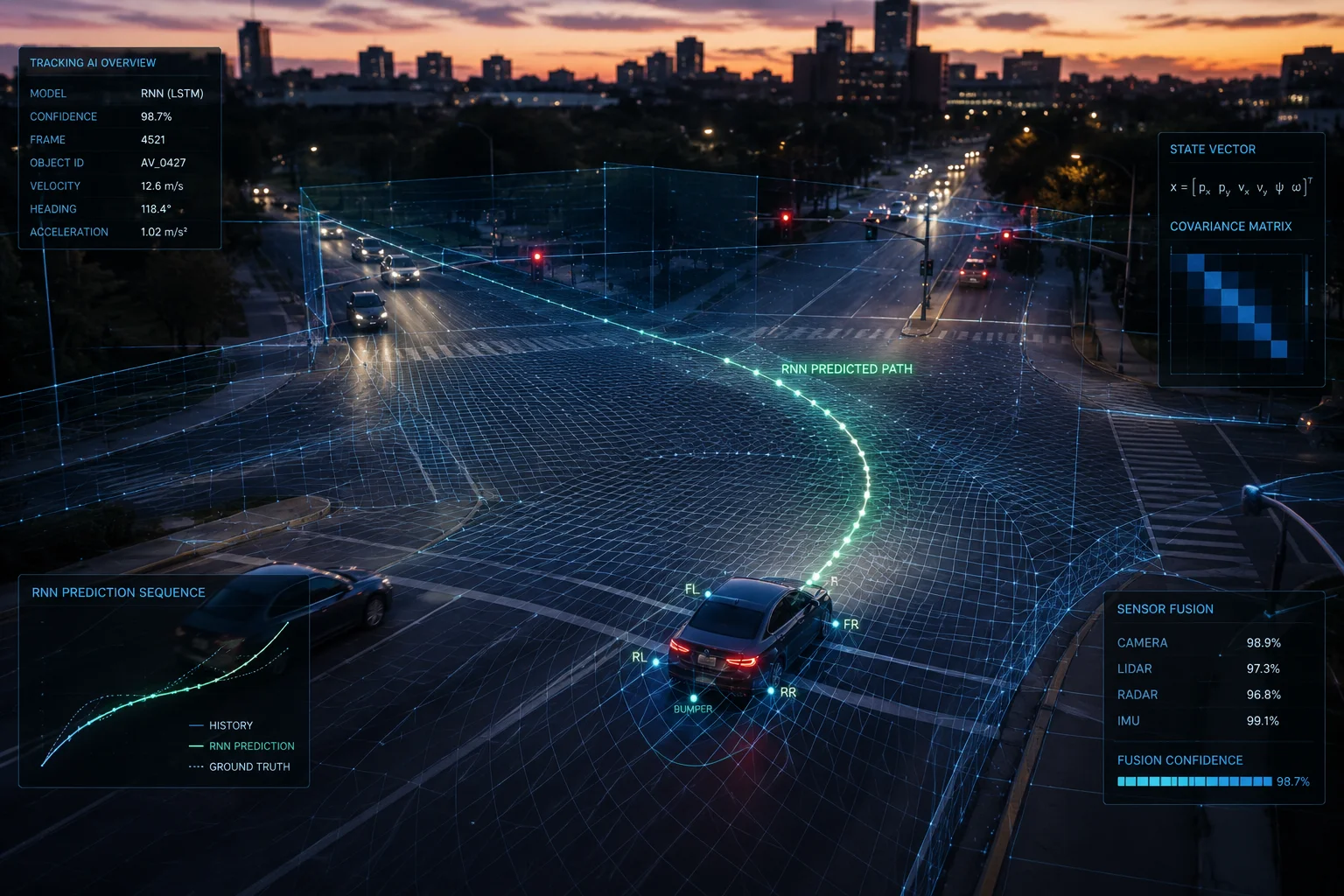 vehicle non-linear speed trajectory prediction PTZ
Why Vehicles Break Simple Prediction Models
A basic linear prediction assumes constant velocity. If a car is going 40 km/h heading east, it predicts the car will still be going 40 km/h heading east in one second. But vehicles don’t work that way. They brake for intersections. They accelerate onto highways. They curve around bends.
A pure Kalman Filter improves on this by modeling acceleration. It can handle smooth speed changes. But it still struggles with sudden events like hard braking or sharp turns.
The Hybrid Approach: Kalman + RNN
Our system uses both models together:
Kalman Filter role: Handles the physics. Tracks position, velocity, and acceleration in real-time. Updates predictions every frame (33ms at 30fps). Very fast, very efficient on embedded hardware.
RNN role: Handles the behavior. It has been trained on thousands of hours of vehicle movement data. It recognizes patterns that pure physics can’t predict. For example:
- A vehicle slowing down near an intersection will likely stop or turn
- A vehicle on a straight road with no obstacles will likely maintain speed
- A vehicle that has been accelerating for 3 seconds will likely reach a cruising speed soon
Real-World Performance Numbers
In our testing across different scenarios:
A vehicle accelerating from 0 to 60 km/h: the prediction stays within 2 meters of actual position throughout the acceleration phase. The system recognizes the acceleration pattern within 500ms and adjusts its model.
A vehicle braking suddenly: the prediction overshoots by about 3-4 meters initially, but corrects within 300ms. The camera never loses the vehicle because the field of view at typical tracking zoom levels covers this error margin.
A vehicle turning at an intersection: this is the hardest case. The RNN detects the deceleration pattern that precedes a turn and begins adjusting the predicted path before the turn actually starts. Success rate for maintaining lock through a 90-degree turn is about 85%.
Practical Advice for Vehicle Tracking Deployments
For David and other integrators deploying vehicle tracking: set the prediction model to “Vehicle Mode” in the firmware settings. This switches the RNN to a vehicle-specific weight set and increases the Kalman Filter’s acceleration tolerance. The system will be less sensitive to sudden speed changes and won’t interpret hard braking as “target lost.”
Also, consider mounting height. For vehicle tracking, a higher mount (8-12 meters) gives the algorithm better depth estimation because the angle between camera and ground plane is more favorable for 3D mapping.
Conclusion
3D trajectory prediction turns a PTZ camera from a reactive follower into a proactive tracker. It handles blind spots, compensates for 4G latency, smooths motor movement, and adapts to non-linear vehicle speeds. For any serious long-range deployment, this is the feature that separates professional results from frustrating failures.
1. Overview of trajectory prediction methods in robotics and control systems. ↩︎ 2. Detailed explanation of the Kalman filter algorithm used for state estimation and prediction. ↩︎ 3. Overview of behavior modeling using deep learning for trajectory prediction. ↩︎ 4. Basics of RNNs and their application in sequence prediction tasks. ↩︎ 5. Overview of geographic coordinate systems used in spatial mapping. ↩︎